Pivot Table - Customizing and Formatting

Sum or Count
When creating a pivot table, Excel will automatically sum or count the items. If all the cells in a column contain numeric data, Excel chooses to sum. However, if one cell is either blank or contains text, Excel will choose to count.

To overwrite the default:

Right click any cell of the column that need to be changed, from the drop-down list, choose "Summarize Values By", from the fly-out menu click "Sum", then the pivot table will sum the items as follows:

Replacing Blanks with Zero
By default, pivot table will leave empty cells blank. To avoid values columns been treated as text just because of one blank cell, we can replace the blank cells with zeros:

Right click any cell of that specific column, choose Pivot Table Options:

A "Pivot Table Options" window will be activated:

In the pop up window, under Layout and Format tab, go to Format, type "0" into the box next to the field "For empty cells show".

Grand Totals
The default in Pivot Table is to show "Grand Total" for both rows and columns:

If user just want Grand Total rows, but not Grand Total columns, that can be done as follows:

Go to Design tab => Select Grand Totals =>Select "On For Rows Only" from the drop-down list

The drop-down list offers 4 choices, users can also choose "On for Columns Only", or on and off for both.


Subtotals
There are times users need to suppress the subtotals. To do so, user can go to Design tab, then

click Subtotals, from the drop-down list, select Do Not Show Subtotals.

However, this action will turn off all Subtotals. If user only want to suppress subtotals for particular column(s), then place the cursor in any cell of that particular column, go to Analyze tab, select Field Settings

 Field Settings dialog box will then pop up:

Change the Subtotals setting from "Automatic" to "None" as above.

 

Report Layouts
Compact Layout is the default Pivot Table report layout:

The compact form is suited for using the Expand and Collapse icons, by clicking the plus icons, users can expand and collapse to view and hide the details. However, if users want to do some subsequent analysis, they will want each row field in a separate column, which means an Outline Layout or a Tabular Form may be a better choice.

 To change the Report Layout, go to Design tab, select Report Layout, from the drop-down list, select Show in Tabular Form:

Pivot Table Basics - Calculated Fields

Users often need to perform data based calculations that are not in the original data set. This can be done in pivot table through the "Calculated Field". A calculated field is a virtual data field created by executing a calculation against existing fields in the pivot table, just like a new virtual column added to the data set.

Next, we will add a calculated field to the following pivot table:

Create a Calculated Field

Steps to create a calculated field:

(i) Select "Analyze" under the Pivot Table Tools
(ii) Select "Fields, Items & Sets"
(iii) From the drop-down menu select "Calculated Field".

(iv) The "Insert Calculated Field" dialog box will pop up

There are two input boxes inside the dialog screen. At the top is the "Name" field, which user can name the calculated field with a name of their choice, better appropriately to meet its function.

The one below is the "Formula" box, user can build their own formula by selecting the combination of data fields from the underneath "Fields" list box.

In this example, we create a calculated field to calculate the "Profit" for the property transactions:

We first select and double click the "Selling price" field, then enter the mathematical operator "- ", follow by "Purchase price"; then repeat the process again for each of the cost items to finalize the following formula into the formula box:

"Selling Price"-"Purchase Price"-"Stamp Duty"-"Conveyance"-"Improvement Cost"

Finally, click "O.K"

Then we can see the field under the name of "Sum of Profit" been added to Pivot Table:

Once the new calculated field was created, we can also find it in the "Fields" list box:

Pivot Table - Data Model

Data Model is an in-memory analytics tool introduced by Microsoft since Excel 2013, which can be used to work with disparate data.

Up to this point, we have been working with source data from one table. In reality, users will most likely encounter data from disparate data source. Start from the basic again, in the following example we are working with data source from two tables within the same worksheet:

The table on the left is a Sales summary, and the one on the right is a Salesperson table, we want to group them together to find out the performance of the salespersons.

First, we need to tell Excel their relationship, and then pull them into the internal Data Model.

Step 1: Click any cell of the Sales Summary table.

Step 2: Go to ribbon, select "Insert"

Step 3: Select "Pivot Table"

Step 4: "Create Pivot Table" dialog box will pop up

Step 5: Select and check the range, select "New Worksheet"

Step 6: Be sure to check next to the "Add this data to the Data Model" => OK

Step 7: Click any cell inside the Salesperson table

Step 8: Repeat the procedure (Step 2 to 5) for the Salesperson table.

Step 9: On the "Create Pivot Table" dialog box, also  check the box next to the "Add this data to the Data Model"

Underneath the "Pivot Table Fields", we can see there's an "Active" and "All" , we select "All".

"Range" and "Range 1" is the two tables of our source data.

We can click the arrowhead to the left of "Range" and "Range 1" and select fields to incorporate into our new Pivot Table.

We select "Salesperson" to Rows and "Amounts" to Values.

Excel recognises that we are using two tables from our Data Model, and prompts us to create a relationship between them.

To set up the relationship, we click "CREATE"

This is the crucial part, we have to let Excel know the relationship between the two tables, then Excel will base on this relationship to build up the Pivot table. In our example, their relationship is linked by the customers, which is also the common attributes in both tables.

Therefore, we linked up the "Customers" from Sales summary table to the "Cust." in the Salesperson table as shown in the "Create Relationship" dialog box per above.

Following is the resulting Pivot table:

Pivot Table - Basic

Pivot Table is commonly used to extract, summarize and analyze data. With a pivot table, user can transform numerous rows of data into a concise summary report within seconds.

Let's start from the basic, walk through a simple example, using the following table as our data source to construct a Pivot table.

Create Pivot Table

Click any cell inside the source data table.

Then, go to ribbon, select "Insert" tab.

Under Insert tab, select "Pivot Table"

The "Create Pivot Table" dialog box will pop up.

It has already pre-selected the source data range. Check to ensure the whole data source table has been included.

Then, select "New Worksheet" for our Pivot Table.

In the new worksheet for the Pivot Table, we can see that it is still a blank worksheet. There is no Pivot table yet. That's because user have to tell Excel what to include in the Pivot table and how should the Pivot table be presented. These can all be done in the "Pivot Table Fields" box.

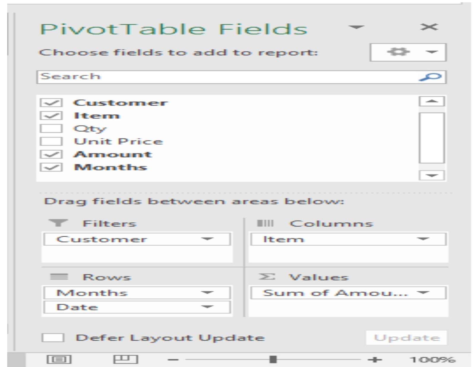
"Pivot Table Fields" box is located on the right hand side of the new worksheet. It is through this box user tells Excel how the pivot table should be constructed.

The "Pivot Table Fields" box has two sections. The top part is the Fields section, and the bottom part is the Area section.

The Fields section contains all the fields of the original data table, and user can select any fields to be used in the new pivot table, just by checking the box next to the field name.

The Area section is for users to decide how to arrange those selected fields. There are four small boxes in the Area section: "Filters", "Columns", "Rows" and "Values".

Placing a data field in the "Columns" area will display the data in a column-oriented perspective, with headings stretch across the top of the columns in the new pivot table.

"Rows" area fields are displaying as rows in the new pivot table.

The "Values" area calculates and counts data. The data field that you drag and drop there are typically that you want to measure.

"Filters" area is an optional set of one or more drop list at the top of the pivot table. Placing data fields into the "Filters" area allows users to filter the entire pivot table based on selections. The types of data field that you might drop there should be those that you want to isolate or focus on; for example, customers, products or employees.

Once user checking the field lists in the "Fields" section, Excel will automatically allocate the fields to Area section. By default, Excel will automatically place non-numeric fields to the "Rows" area, numeric fields are added to the "Values" area, Date and time will be added to "Columns" area. Of course, users can always drag the fields between areas to customize out their own pivot table.

As an example, we select four fields:
Customer/Item/Amount/Months, drag and place them into the following boxes of the Areas section:

Customer -> Filters
Items -> Columns
Date -> Rows
Amount ->Values






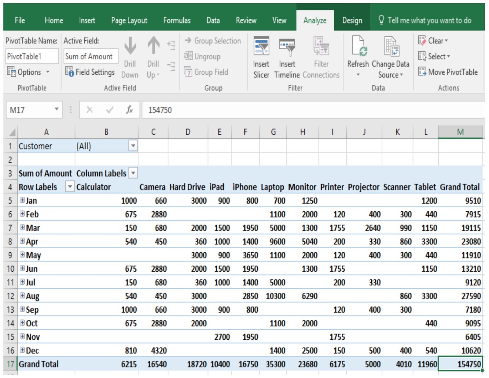
Following is the resulting pivot table:

As "Customer" is the Filters, we can use the filter button at B1 to select any particular customer for our review.

In order to check the table is properly produced, we first select "All" at "B1" to compare the total of our Pivot Table with the original data table, both giving $151,745 as the Grand total.

From the resulting pivot table, we can see that with a pivot table, users can quickly categorize unorganized data into groups of meaningful data.

By using a pivot table, the original data set doesn't have to be changed, but the pivot table itself can be changed dynamically to do different analyses based on user's specifications, and interactively drilled down to detailed records.

In our example, the pivot table helps us to have a clear picture of our sales by product on a monthly basis. And, by clicking the filter button at B1, we can also select individual customers to see how we perform towards each of them. In the following table, we select customer "DEF" at B1, the resulting table shows how we perform towards them in last calendar year.

Grouping Dates

With Excel 2016, Microsoft has added some new features for grouping, sorting, and filtering. Grouping dates is one of those new features.

In our Pivot table, all dates have been automatically grouped into their respective months.

By clicking the plus(+) icon of the respective month, Excel will expand that month to show the detailed transactions by dates. In our table, we select to show the detailed transactions in January.


Data Changed

(A) Pivot Table needs to be "Refresh" each time the source data has changed



In our example, we have made some changes to the source data.

New unit prices been used for products on Row 92 to Row 100, which in terms also affected the respective sales amount and the grand total of the whole table.

 

To update the change, click any cell inside the Pivot Table. Go to Ribbon, select "Analyze" -> "Refresh" -> "Refresh"

After "Refresh", the pivot table is updated, as can be seen from the new grand total.

(B) If source size varies (i.e. adding or deleting rows/columns), user has to re-define the range of source data



In our example, we add 5 rows to our source data table.

To update, right click any cell inside Pivot Table. Go to ribbon, select "Analyze" -> "Change Data Source" -> "Change Data Source"

 

 

Once we click "Change Data Source", Excel will bring us back to the original worksheet of the data source table, and the "Change Pivot Table Data Source" dialog box will pop up as shown above.

 

The dialog box will first pre-select the range of the old data source, this must be changed to include the new additions, and click "OK" to update the new range.

 



Following is the updated Pivot Table: